Spherical Harmonics for Environment Map Lighting with PyTorch3D

This post explores a practical method for using spherical harmonics in scene illumination. Instead of directly calculating light from spherical harmonics, we’ll convert them into a 2D UV environment map for efficient sampling. This approach transforms spherical harmonics into 2D image that can be easialy understood, analyzed and regularized. Don`t forget to run the code in google colab to try it all by yourself.

Spherical Harmonics in Illumination

• Brief introduction to spherical harmonics
• Advantages in representing lighting environments

Imagine wrapping your entire scene in a giant bubble. Now, picture that this bubble isn’t just plain - it’s covered in a complex pattern of light and color. That’s essentially what spherical harmonics help us do in computer graphics. Spherical harmonics are like a special set of building blocks. Just as you can build complex Lego structures with a few basic pieces, we can describe intricate lighting patterns using these mathematical building blocks. To figure out what’s happening at any point on our imaginary bubble, we use two simple measures:

How far up or down the point is (that’s our polar angle, $\theta$) How far around the bubble we’ve gone (that’s our azimuth angle, $\phi$)

With just these two pieces of information, we can map out the entire lighting environment surrounding our scene. It’s like creating a super-efficient light map that tells us how bright and what color the light is coming from every direction. The best part? This method gives us a compact way to store all this lighting info. Instead of trying to remember every tiny detail about the light, we just need to keep track of a few key numbers. It’s like compressing a huge image file into a small, manageable size, but for lighting!

Representation of spherical harmonics on the sphere

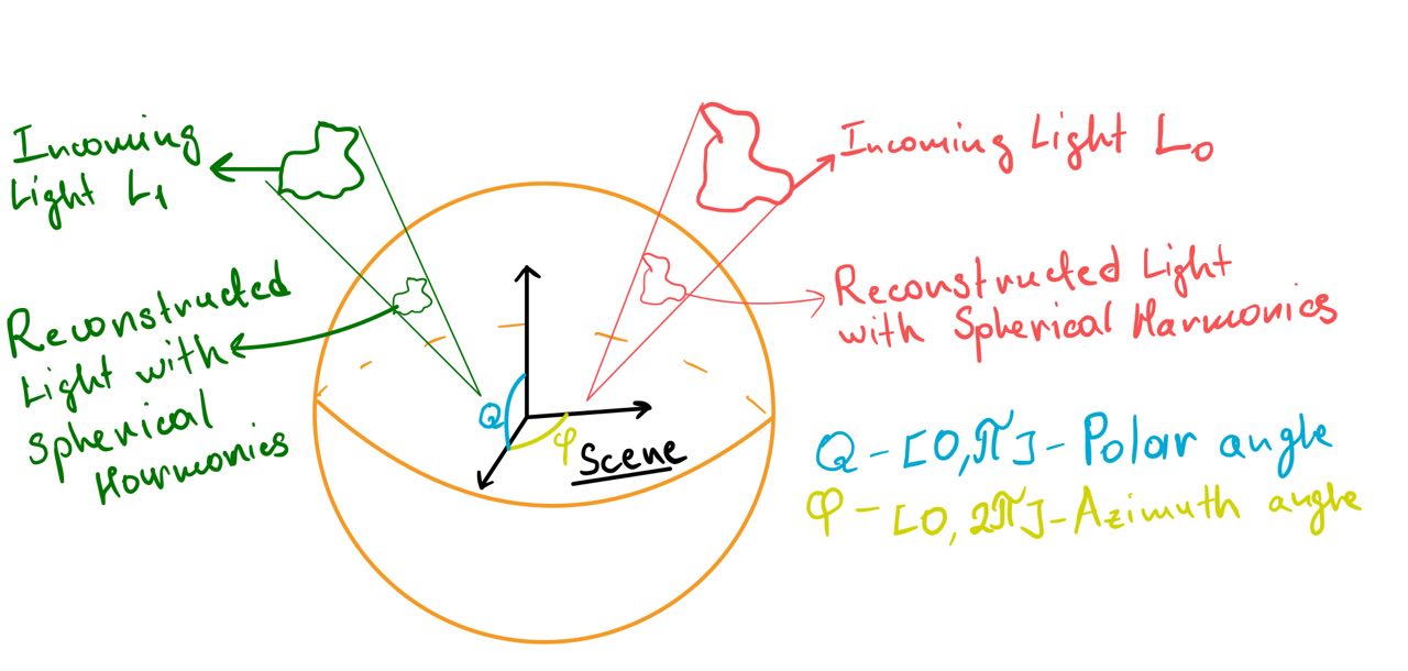
On the image above our scene is surrounded by this sphere. We have two light sources: $L_0$ (a red light pattern) and $L_1$ (a green light pattern). We can actually model these two light sources on the sphere surface by finding the right set of spherical harmonics coefficients. Let’s take a closer look at the math behind this.

Converting Spherical Harmonics to Environment Maps

• Mathematical overview
• Implementation using PyTorch

Spherical Harmonic basis functions

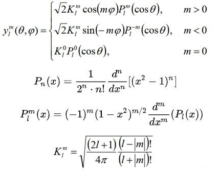
For people who can read this high level math here is some brief annotation:

1. $y_l^m(θ, φ)$: Spherical harmonic function of degree l and order m. The degree l determines the overall complexity, while the order m (ranging from -l to l) specifies the number of azimuthal oscillations around the sphere.
2. $θ, φ$: Spherical coordinates (polar angle, azimuthal angle)
3. $K_l^m$: Normalization factor ensuring orthonormality of spherical harmonics.
4. $P_l^m$: Associated Legendre polynomial, defining the θ (polar) oscillation pattern and frequency.
5. $\cos(m \phi), \sin(m\phi)$: $\phi$ - dependent terms, creating azimuthal variation. These functions control the SH’s oscillation around the equator, with $m$ determining the frequency of these azimuthal oscillations.

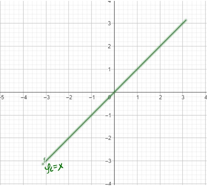
For other people who want to see light in the end of this chapter lets first understand concept of basis functions and where they used. Imagine we have a function to approximate:

This is one of the simplest functions we`ve studied back in school. As our basis let`s choose periodic function:

Our goal is to approximate $\phi_{t}$ as a linear combination of these basis functions:

The process of finding coefficients $a_0, a_1, a_2, …$ is called the Fourier Series Expansion. It works by decomposing the target function into a sum of sine and cosine functions(in our example we use only sine functions) - orthogonal basis functions—and finding the coefficients by projecting the target function onto each basis function through integration. For sake of simplicity we consider interval $x \in [-\pi, \pi]$. We won`t go into details towards how this coefficients is found, but lets see how with each new basis added we getting better approximation of our target function $\phi_{t}$.

Target function: $\phi_{t}(x) = 2\sin(x)$

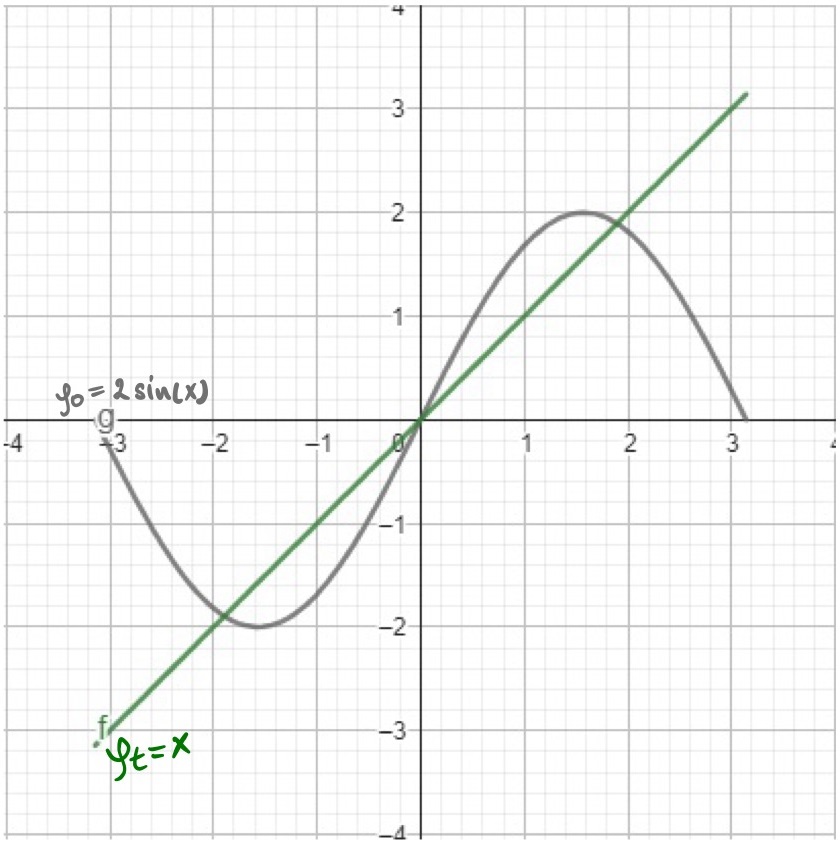
Using the Fourier Series Expansion out first coefficient $a_0=2$, so our 0-th approximation is $\phi_0(x) = 2\sin(x)$. As we can see on the image bellow $\phi_0(x)$ is doing a bit poor job approximating our target function. Let`s throw into the mix second basis function $a_1\sin(2x)$ and see how it will improve our approximation. The second order approximation is $\phi_1(x) = 2\sin(x) - \sin(2x)$. The countour of the function is getting closer to our target function.

First approximation: $\phi_0(x) = 2\sin(x)$

Second approximation: $\phi_1(x) = 2\sin(x) - \sin(2x)$

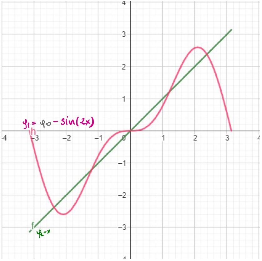
Step by step adding new basis $\phi_2, \phi_3, \phi_4$ with coefficients $a_2=\frac{2}{3}, a_3=-\frac{1}{2}, a_4=\frac{2}{5}$ we getting better and better approximation of our target function. Each approximation occilates more frequently around the target function making approximation more accurate.

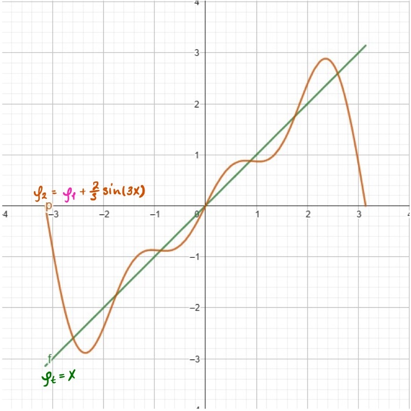
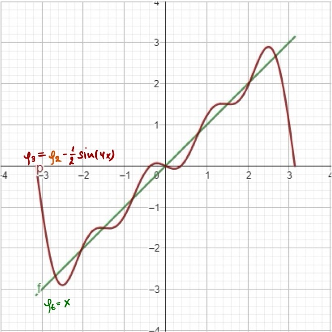
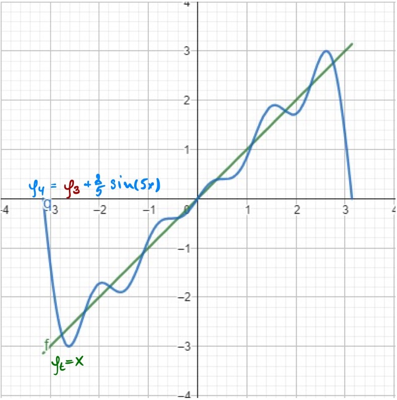
Next order approximations: $\phi_3(x)$, $\phi_4(x)$, $\phi_5(x)$

Approximation of $\phi_t(x)$ with 30 basis functions

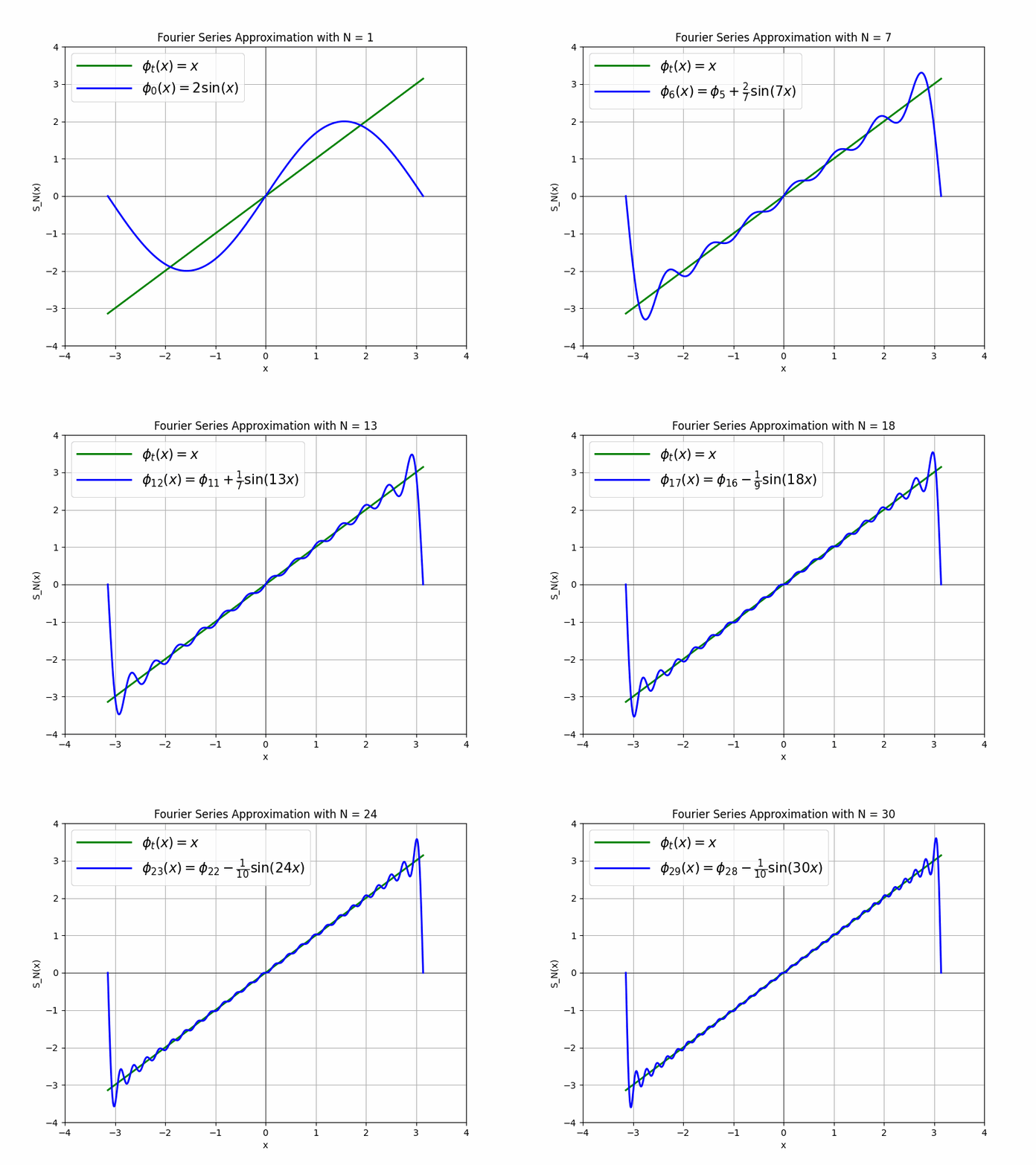
What is cool about this approch is how we just threw in new basis function with new coefficients without recalculating all the previous ones. This is the power of ORTHOGONALITY. Because basis function does not influence each other we can just add new ones and find their coefficients INDEPENDENTLY. For us, computer people this word translates into parallelization. We can speed up our computations and also reuse previous iterations, nothing goes to waste. This is the same property that Spherical Harmonics poses. Those tricky formulas actually generate infinite set of basis functions that are orthogonal between each other. SH basis functions can be used to approximate any function on the surface of the sphere. In our practical case is a lighting pattern around our scene. Hopefully, orthogonality property of SH is more or less clear now, but what about those degree and order?

Spherical Harmonics Bands

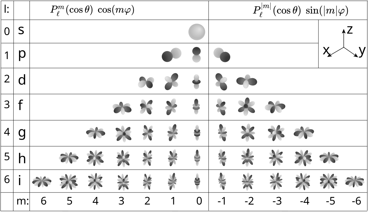
On the image above you can observe different SH bands. With each new degree $l$ we add new band of functions. Order $m$ describes number of oscillations within each band and ranges $[-l, l]$. New band provides more variability and allows us to represent more complex patterns. In case of using SH for representing lighting patterns we usually limit ourselves with degree $l=2$. This is because lighting patterns are usually smooth and do not require high frequency oscillations. For degree $l=2$ we have 9 basis functions in total. Why 9? because total number of basis functions is $1 + 3 + 5 = 9$ - first 3 rows of the image above. Enought of math for now, let`s focus on how we can code these equations and see what patterns they represent. There are 2 common ways to approach calculation of light with spherical harmonics:

Direct Evaluation - having a direction represented as two angles ($θ$(polar), $φ$(azimuthal)) just throw in coefficients and input angles into the equation and receive lighting value.

Precompute Environment Map - at first generate a grid of ($\theta - [0, \pi], \phi - [0, 2\pi]$). The resolution of Environment Map is up to you and controlled by sampling density. Then for each grid points we calculate a light value using SH coefficients and get Environment Map as 2d image which we can observe, interprete and analyze.

Direct Evaluation is more suitable for real-time applications where we need to compute lighting for each point on the fly. Precompute Environment Map is more suitable for offline rendering tasks where we can afford to preprocess the lighting data and use it for real-time rendering. In our case we will focus on the second approach as its more visual and suitable for understanding.

At this point, all we want is to hide these SH equations inside the class which do everything, so we don`t need to think about what`s going on there ever again.

First step is create small function to set the resolution for the Env Map and compute $\theta$ and $\phi$ grids. There is a little trick here with adding 0.5 to the uv grid during remapping from $[0,res]$ to $[0, \pi]$ and $[0, 2\pi]$. This is done, so we calculate SH values for the center of each pixel, not for the corner.

def set_environment_map_resolution(self, res):
  """ Step 1: Set the resolution for the environment map and compute theta and phi grids """
  res = (res, res)
  self.resolution = res
  uv = np.mgrid[0:res[1], 0:res[0]].astype(np.float32)  # ranges [0, res]
  self.theta = torch.from_numpy((math.pi / res[1]) * (uv[1, :, :] + 0.5)).to(self.device)  # Theta ranges from [0, pi]
  self.phi = torch.from_numpy((2 * math.pi / res[0]) * (uv[0, :, :] + 0.5)).to(self.device)  # Phi ranges from [0, 2*pi]

Second step is to write a function to calculate associated Legendre polynomials. They have recursive relationship which we can use to compute them. Code for this is kind of counterintuitive, but it follows the definition $P_l^m$.

Associated Legendre polynomial

def compute_associated_legendre_polynomial(self, l, m, x):
    """ Step 2: Compute the associated Legendre polynomial P_l^m(x) """
    # P_m^m(x): Base case for the recursion, where l == m
    pmm = torch.ones_like(x)
    if m > 0:
        somx2 = torch.sqrt((1 - x) * (1 + x))  # sqrt((1 - x) * (1 + x))
        fact = 1.0
        for i in range(1, m + 1):
            pmm = pmm * (-fact) * somx2  # Recursively compute P_m^m(x)
            fact += 2.0
    if l == m:
        return pmm
    
    # P_m^(m+1)(x): Next step in the recursion
    pmmp1 = x * (2.0 * m + 1.0) * pmm
    if l == m + 1:
        return pmmp1
    
    # P_l^m(x): General case for l > m
    pll = torch.zeros_like(x)
    for ll in range(m + 2, l + 1):
        pll = ((2.0 * ll - 1.0) * x * pmmp1 - (ll + m - 1.0) * pmm) / (ll - m)  # Recurrence relation
        pmm = pmmp1
        pmmp1 = pll
    return pll

Third step: Normalization factor

Fourth step: Spherical harmonic formula

def compute_normalization_factor(self, l, m):
    """ Step 3 Compute the normalization factor for the spherical harmonic function """
    # Normalization factor to ensure orthonormality of the spherical harmonics
    numerator = (2.0 * l + 1.0) * math.factorial(l - m)
    denominator = 4 * math.pi * math.factorial(l + m)
    return math.sqrt(numerator / denominator)

def evaluate_spherical_harmonic(self, l, m, theta, phi):
    """ Step 4: Evaluate the spherical harmonic function Y_l^m for given theta and phi """
    # Evaluate Y_l^m based on whether m is positive, negative, or zero
    if m == 0:
        return self.compute_normalization_factor(l, m) * self.compute_associated_legendre_polynomial(l, m, torch.cos(theta))
    elif m > 0:
        return math.sqrt(2.0) * self.compute_normalization_factor(l, m) * \
                torch.cos(m * phi) * self.compute_associated_legendre_polynomial(l, m, torch.cos(theta))
    else:
        return math.sqrt(2.0) * self.compute_normalization_factor(l, -m) * \
                torch.sin(-m * phi) * self.compute_associated_legendre_polynomial(l, -m, torch.cos(theta))

Last but not least, we need to iterate over all basis functions and compute their values for each grid point.

def construct_environment_map_from_sh_coeffs(self, sh_coeffs, smooth=False):
    """Construct an environment map from the given spherical harmonic coefficients """
    ...
    # Loop through each band and order to compute the environment map
    for l in range(bands):
        for m in range(-l, l + 1):
            sh_value = self.evaluate_spherical_harmonic(l, m, theta, phi)
            result = result + sh_value.view(sh_value.shape[0], sh_value.shape[1], 1) * smoothed_coeffs[:, i]
            i += 1

    # Ensure non-negative values in the result
    result = torch.max(result, torch.zeros(res[0], res[1], smoothed_coeffs.shape[0], device=smoothed_coeffs.device))
    ...

To see the whole SphericalHarmonics class implementation, refer to the notebook code. With this class we can now generate environment map from the given SH coefficients, but now comes more 3D Graphics stuff.

Scene Illumination with Environment Maps

• Calculating specular reflections
• Calculating diffuse lighting
• Sampling the Environment Map

To render the scene with 2D Env Map we are going to use PyTorch3D library. It provides a lot of useful tools for 3D graphics tasks. We are going to use MeshRenderer, SoftPhongShader and FoVPerspectiveCameras to render our scene. Pytorch3D library provides different types of lighting schemes - PointLights, DirectionalLights, AmbientLights and SpotLights. But to use our new Environment Map generated from SH, we are going to implement our own lighting class EnvMapLights.

When light interacts with the surface of an object, it can be reflected in different ways:

• Specular reflection - light is reflected in a specific direction, creating a shiny or mirror-like appearance.
• Diffuse reflection - light is scattered in all directions, creating a diffuse appearance.

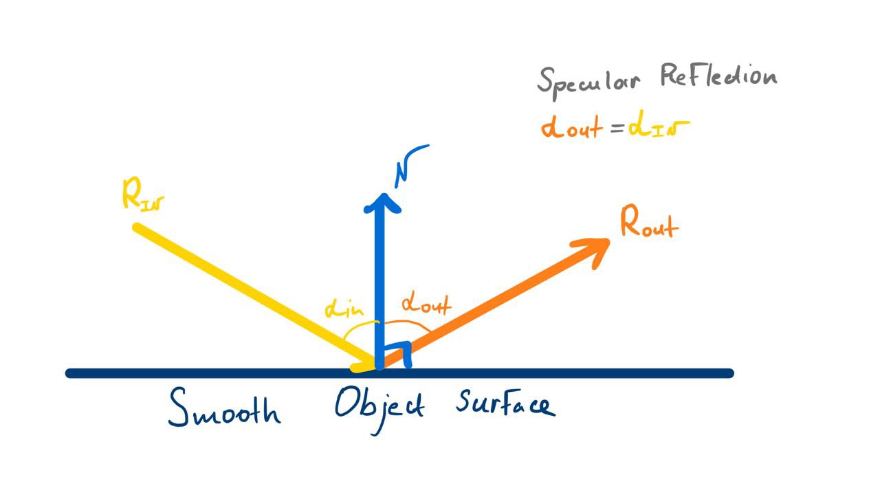
Specular reflection is responsible for creating highlights and shiny surfaces. Incoming light rays $R_{\text{in}}$ bounces off the surface and becomes $R_{\text{out}}$. $R_{\text{out}}$ has the same angle to surface normal $N$ as $R_{\text{in}}$. To calculate $R_{\text{out}}$ we need to reflect $R_{\text{in}}$ over the surface normal $N$. We will use newly calculated $R_{\text{out}}$ to sample lighting value from the Environment Map.

Specular reflection

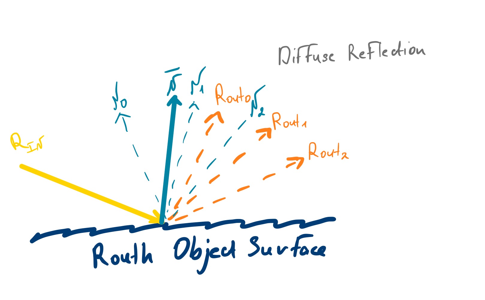
Diffuse reflection is responsible for creating a diffuse appearance. In this case, light is scattered in all directions, creating a uniform illumination across the surface. Due to the roughness of the surface incoming rays $R_{\text{in}}$ are reflected in different directions. Instead of modeling each ray reflection depending on the point it hits, we just use the normal $\overline{N}$ average of $N_0, N_1, N_2$. $\overline{N}$ nicely describes small region of the surface and used to sample lighting value from the Environment Map. It will provide average lighting value of rays scattered across that surface region.

Diffuse reflection

To sample values from Environment Map for specular reflection use $R_{\text{out}}$ direction and for diffuse reflection use normal $\overline{N}$. Now the question is how having 2 direction vectors get light values from 2D map images. It is actually quite simple:

1. Convert $(x,y,z)$ euclidian direction vector to spherical coordinates ($\theta, \phi$);
2. Normalize $\theta$ and $\phi$ to uv coordinates in $[0, 1]$ range;
3. Use uv coordinates to sample lighting value from the Environment Map.

But because we are lazysmart we`ll skip the intermediate convertion to $\theta$ and $\phi$ and directly convert $(x,y,z)$ to uv coordinates. $[-1, 1]$ range is needed as torch.nn.functional.grid_sample expects input mapped in this range.

def _convert_to_uv(self, directions):
    # Calculate the square of each component (x, y, z+1)
    x2 = directions[..., 0] ** 2
    y2 = directions[..., 1] ** 2
    z2 = (directions[..., 2] + 1) ** 2

    # Compute the scaling factor 'm'
    # 'm' is twice the square root of the sum of the squares of the x, y, and z+1 coordinates
    m = 2 * torch.sqrt(x2 + y2 + z2)[..., None]

    # Scale the x and y coordinates by 'm' to normalize them
    uv_directions = directions[..., :2] / m

    # Shift the normalized coordinates to the [0, 1] range by adding 0.5
    uv_directions = uv_directions + 0.5

    # Rescale the coordinates to the [-1, 1] range
    uv_directions = uv_directions * 2 - 1

    return uv_directions

Implementation with PyTorch3D

• Overview of the EnvMapLighting class
• Integration with PyTorch3D’s rendering pipeline
• Optimizing Environment Map Lighting via Spherical Harmonics coefficients

EnvMapLighting class is in Pytorch3D library style implements two main methods:

1. def diffuse(self, normals, points=None):
2. def specular(self, normals, points, camera_position, shininess):

In EnvMapLighting.diffuse method we use normals of the surface, convert them to uv coordinates in $[-1, 1]$ range and sample lighting value from the Environment Map.

def diffuse(self, normals, points=None) -> torch.Tensor:
        """
        Calculate the diffuse component of light reflection using Lambert's
        cosine law.

        Args:
            normals: (N, ..., 3) xyz normal vectors. Normals and points are
                expected to have the same shape.
            color: (1, 3) or (N, 3) RGB color of the diffuse component of the light.
            direction: (x,y,z) direction of the light

        Returns:
            colors: (N, ..., 3), same shape as the input points.
        """
        ...
        # Renormalize the normals in case they have been interpolated.
        # We tried to replace the following with F.cosine_similarity, but it wasn't faster.
        normals = F.normalize(normals, p=2, dim=-1, eps=1e-6)
        uv_normals = self._convert_to_uv(normals)

        # Convert color from (B, H, W, 1, 3) to (B, 3, H, W) for sampling
        # Convert uv normals from (B, H, W, 1, 2) to (B, H, W, 2)
        input_color = color.squeeze(-2).permute(0, 3, 1, 2)
        grid_uv_normals = uv_normals.squeeze(-2)

        sampled_color = torch.nn.functional.grid_sample(input_color, grid_uv_normals, padding_mode="reflection", align_corners=False)
        ...

In EnvMapLighting.specular method a bit more steps as at first $R_{\text{out}}$ is calculated and then converted to uv coordinates.

def specular(self, normals, points, camera_position, shininess) -> torch.Tensor:
    """
    Calculate the specular component of light reflection.

    Args:
        points: (N, ..., 3) xyz coordinates of the points.
        normals: (N, ..., 3) xyz normal vectors for each point.
        direction: (N, 3) vector direction of the light.
        camera_position: (N, 3) The xyz position of the camera.
        shininess: (N)  The specular exponent of the material.

    Returns:
        colors: (N, ..., 3), same shape as the input points.
    """
    ...
    normals = F.normalize(normals, p=2, dim=-1, eps=1e-6)
    # Calculate the specular reflection.
    view_direction = camera_position - points
    view_direction = F.normalize(view_direction, p=2, dim=-1, eps=1e-6) # R_in

    cos_angle = torch.sum(normals * view_direction, dim=-1)
    # No specular highlights if angle is less than 0.
    mask = (cos_angle > 0).to(torch.float32)


    reflect_direction = -view_direction + 2 * (cos_angle[..., None] * normals) # R_out
    reflect_direction = torch.nn.functional.normalize(reflect_direction, dim=-1) # R_out

    uv_reflect_direction = self._convert_to_uv(reflect_direction)
    # Convert color from (B, H, W, 1, 3) to (B, 3, H, W) for sampling
    # Convert uv reflect directions from (B, H, W, 1, 2) to (B, H, W, 2)
    input_color = color.squeeze(-2).permute(0, 3, 1, 2)
    grid_uv_reflect_direction = uv_reflect_direction.squeeze(-2)

    sampled_color = torch.nn.functional.grid_sample(input_color, grid_uv_reflect_direction, padding_mode="reflection", align_corners=False)
    # Convert from sampled color (B, 3, H, W) to (B, H, W, 1, 3) like normals dims
    color = sampled_color.permute(0, 2, 3, 1).unsqueeze(-2)
    ...

The shininess parameter in the EnvMapLighting.specular method controls the sharpness and intensity of the specular highlights on a surface. It is a fundamental part of the Phong reflection model, which is widely used to simulate how light reflects off a surface.

Having all the puzzle pieces put together we can now reconstruct the scene illumination with Environment Map generated from SH coefficients. I previously generated a training dataset $I_{\text{p}}$ of a cow mesh using 10 different camera angles and a PointLights illumination scheme from PyTorch3D. Now we can use the same camera angles and mesh to recreate the PointLights lighting with our EnvMapLighting class and see it`s capabilities.

Training Images with PointLights illumination

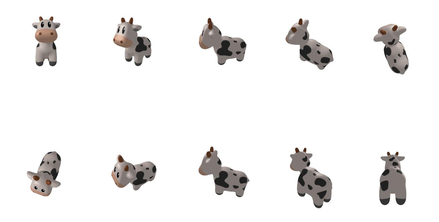
To begin with we have to initialize our SphericalHarmonics class and define the loss function and optimizer. Our resulting Env Map will be a $256 \times256$ image. Usually, to reconstruct scene illumination first 3 bands of spherical harmonics are enough. In most cases scene light is smooth and does not require high frequency oscillations. This means we have $3^2 = 9$ coefficients to optimize. Also, in our experiment we will use 2 sets of coefficients for diffuse and specular lighting seperately to have more control over the lighting. During optimization of SH coefficients we will use simple MSE loss function and Adam optimizer.

sh = SphericalHarmonics(256, device='cuda:0')

batch_size = 1
sh_coeffs = 9 # order 3
learning_rate = 0.02
num_epochs = 300  # Adjust as needed

# Initialize coefficients
diffuse_sh_coefs = torch.ones((batch_size, sh_coeffs, 3), device='cuda:0')
diffuse_sh_coefs.requires_grad = True


specular_sh_coefs = torch.ones((batch_size, sh_coeffs, 3), device='cuda:0')
specular_sh_coefs.requires_grad = True

# Define loss function and optimizer
loss_function = torch.nn.MSELoss()
optimizer = torch.optim.Adam([diffuse_sh_coefs, specular_sh_coefs], lr=learning_rate)

But why torch.ones((batch_size, band, 3), device='cuda:0') use 3 sets of coefficients? Because we have 3 channels in our RGB image and we need each set of coefficients for each channel. As a result for diffuse lighting $3 * 9 = 27$ and for specular lighting $3 * 9 = 27$ coefficients. Next step is just to optimize our coefficients in a loop, generate Environment Map from SH coefficients and calculate loss.

for epoch in range(num_epochs):
    optimizer.zero_grad()

    # Generate environment map from spherical harmonics coefficients
    diffuse_envmap = sh.convert_sh_to_environment_map(diffuse_sh_coefs).clip(0, 1)
    specular_envmap = sh.convert_sh_to_environment_map(specular_sh_coefs).clip(0, 1)

    pred_images = renderer(meshes, lights=EnvMapLights(diffuse_color=diffuse_envmap,
                                                       specular_color=specular_envmap,
                                                       device=device), materials=materials, cameras=cameras)
    loss = loss_function(pred_images, images)

    # Backpropagation and optimization step
    loss.backward()
    optimizer.step()

    if epoch % 10 == 0:  # Print progress every 100 epochs
        print(f'Epoch [{epoch}/{num_epochs}], Loss: {loss.item()}')

Iteration [0/300], Loss: 0.021584568545222282
Iteration [30/300], Loss: 0.01247326284646988
Iteration [60/300], Loss: 0.002377513563260436
Iteration [90/300], Loss: 0.0010528614511713386
Iteration [120/300], Loss: 0.0007361799362115562
Iteration [150/300], Loss: 0.000530929712112993
Iteration [180/300], Loss: 0.00036182499025017023
Iteration [210/300], Loss: 0.00023683365725446492
Iteration [240/300], Loss: 0.00016318858251906931
Iteration [270/300], Loss: 0.00013571616727858782
Iteration [300/300], Loss: 0.000126944956718944
Training finished!

With each iteration loss reduces meaning our coefficients are getting closer to the optimal values. After 300 iterations we can see that our Environment Map is pretty close to the original training images.

Reconstructed Diffuse and Specular Environment Maps

Test Images with Environment Map Lighting

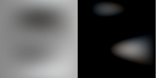
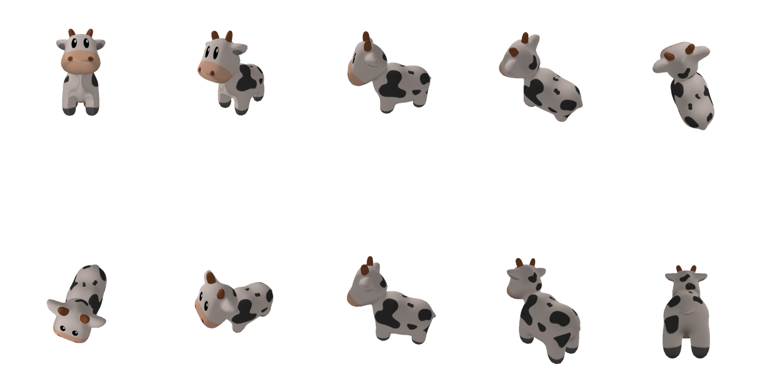
Images above generated with Environment Map Lighting from SH coefficients. We can see that SH coefficents is able to reconstruct the scene illumination with smooth lighting transitions.

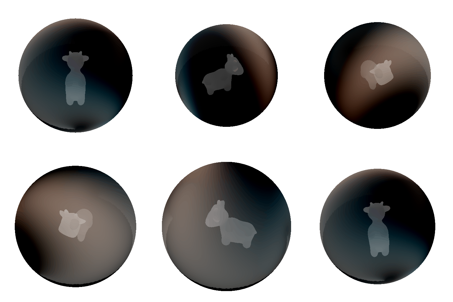
To make one step further, we can zoom out of the scene and orbit around the cow wrapped in the environment map lighting optimized with SH coefficients.

Diffuse Env Map

Specular Env Map

All Together: Lighting with Spherical Harmonics

By combining all the components we’ve discussed, we’ve concocted a magical potion for scene illumination using spherical harmonics! Abracadabra! I hope this all makes sense to you.

And in case not, let’s quickly summarize.

We started by wrapping our scene in a giant bubble and using spherical harmonics as our special set of building blocks to represent complex lighting patterns on its surface. By understanding the concept of orthogonal basis functions—much like in Fourier Series—we saw how we can approximate any function on the sphere’s surface without recalculating previous coefficients.

Next, we converted these spherical harmonics into 2D environment maps. We hid the heavy math inside a handy class that computes associated Legendre polynomials and normalization factors, making it easier to generate and work with these maps.

Then, we explored how light interacts with surfaces through specular and diffuse reflections. By converting our 3D direction vectors directly into UV coordinates, we made sampling from the environment map straightforward and efficient.

Finally, we implemented everything using PyTorch3D. We optimized the spherical harmonics coefficients to match our training images, and with each iteration, our lighting got smoother and more accurate. This demonstrated the effectiveness of using SH coefficients in environment map lighting.

This is it for using spherical harmonics for environment map lighting! I hope this post served you well. Don’t forget to run the code in Google Colab to try it all out yourself. Please don’t hesitate to reach out andask any questions.

Happy rendering!